NASA TurboFan Engine Remaining Useful Life (RUL) Prediction
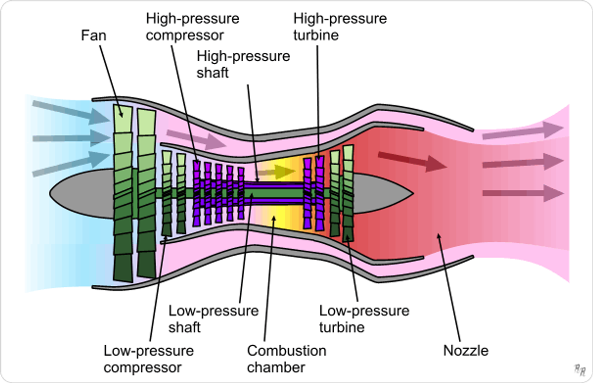
This project is about predicting the Remaining Useful Life (RUL) of NASA's turbofan engines. It is different from my usual business-related projects. However, I believe that by leveraging various tools, machine learning, and deep learning in this project, I can apply similar predictive techniques to forecast future revenues, expenses, and other financial aspects in the accounting and finance departments.
We downloaded the data from Kaggle.
https://www.kaggle.com/datasets/behrad3d/nasa-cmaps
NASA Turbofan Jet Engine Data Set
Run to Failure Degradation Simulation
www.kaggle.com
Data information
About Dataset
Description
Prognostics and health management is an important topic in industry for predicting state of assets to avoid downtime and failures. This data set is the Kaggle version of the very well known public data set for asset degradation modeling from NASA. It includes Run-to-Failure simulated data from turbo fan jet engines.
Engine degradation simulation was carried out using C-MAPSS. Four different were sets simulated under different combinations of operational conditions and fault modes. Records several sensor channels to characterize fault evolution. The data set was provided by the Prognostics CoE at NASA Ames.
Prediction Goal
In this dataset the goal is to predict the remaining useful life (RUL) of each engine in the test dataset. RUL is equivalent of number of flights remained for the engine after the last datapoint in the test dataset.
Experimental Scenario
Data sets consists of multiple multivariate time series. Each data set is further divided into training and test subsets. Each time series is from a different engine i.e., the data can be considered to be from a fleet of engines of the same type. Each engine starts with different degrees of initial wear and manufacturing variation which is unknown to the user. This wear and variation is considered normal, i.e., it is not considered a fault condition. There are three operational settings that have a substantial effect on engine performance. These settings are also included in the data. The data is contaminated with sensor noise.
The engine is operating normally at the start of each time series, and develops a fault at some point during the series. In the training set, the fault grows in magnitude until system failure. In the test set, the time series ends some time prior to system failure. The objective of the competition is to predict the number of remaining operational cycles before failure in the test set, i.e., the number of operational cycles after the last cycle that the engine will continue to operate. Also provided a vector of true Remaining Useful Life (RUL) values for the test data.
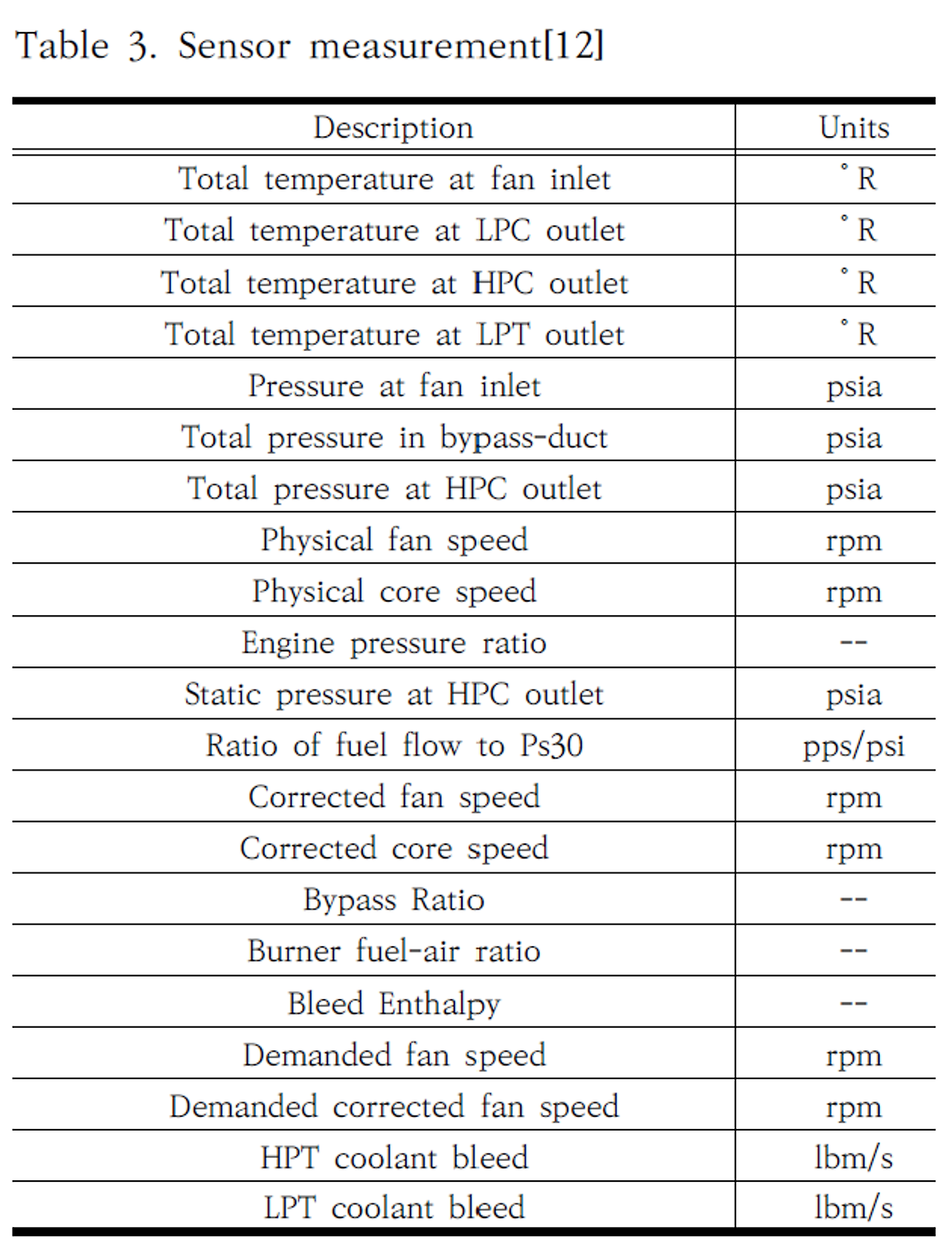
The data are provided as a zip-compressed text file with 26 columns of numbers, separated by spaces. Each row is a snapshot of data taken during a single operational cycle, each column is a different variable. The columns correspond to:
1) unit number
2) time, in cycles
3) operational setting 1
4) operational setting 2
5) operational setting 3
6) sensor measurement 1
7) sensor measurement 2
…
26) sensor measurement 26
Data Set Organization
Data Set: FD001
Train trjectories: 100
Test trajectories: 100
Conditions: ONE (Sea Level)
Fault Modes: ONE (HPC Degradation)
Data Set: FD002
Train trjectories: 260
Test trajectories: 259
Conditions: SIX
Fault Modes: ONE (HPC Degradation)
Data Set: FD003
Train trjectories: 100
Test trajectories: 100
Conditions: ONE (Sea Level)
Fault Modes: TWO (HPC Degradation, Fan Degradation)
Data Set: FD004
Train trjectories: 248
Test trajectories: 249
Conditions: SIX
Fault Modes: TWO (HPC Degradation, Fan Degradation)
Reference
Reference: A. Saxena, K. Goebel, D. Simon, and N. Eklund, Damage Propagation Modeling for Aircraft Engine Run-to-Failure Simulation, in the Proceedings of the 1st International Conference on Prognostics and Health Management (PHM08), Denver CO, Oct 2008.
Alternatively the dataset can be downloaded from https://ti.arc.nasa.gov/tech/dash/groups/pcoe/prognostic-data-repository/
The tools used in this project are as follows:
| Project Name | Description |
| NASA TurboFan Engine Remaining Useful Life (RUL) Prediction | The project's goal is to develop predictive models that accurately estimate the remaining operational time of the engines, leveraging advanced analytical techniques to improve maintenance schedules and operational efficiency |
| Category | Description |
| Language | Python |
| Library | Pandas, Matplotpy, Seaborn, Numpy, sklearn, xgboost, tensorflow |
| Visual Tool | Python, Canva |
import pandas as pd
import seaborn as sns
import matplotlib.pyplot as plt
from sklearn.linear_model import LinearRegression
from sklearn.metrics import mean_squared_error, r2_score
from sklearn.preprocessing import StandardScaler
from sklearn.ensemble import RandomForestRegressor
import xgboost as xgb
import optuna
import numpy as np
from sklearn.preprocessing import MinMaxScaler
from tensorflow.keras.models import Sequential
from tensorflow.keras.layers import LSTM, Dense
from tensorflow.keras.callbacks import EarlyStopping
from tensorflow.keras.preprocessing.sequence import pad_sequences
Project Result
Project Key Points
Data Collection and Preprocessing
- Data preprocessing to ensure the accuracy and reliability of customer data
Approach Sequence:
-
- Data Understanding and Preprocessing
- Understand the structure of the dataset and the meaning of each feature.
- Perform preprocessing such as handling missing values, detecting and dealing with outliers, and normalizing data.
- Feature Engineering
- Extract or transform useful features from engine operational data into a format that can be used as inputs for the models.
- Include extracting cycles from periodic data, computing statistical features, among other techniques.
- Model Selection and Training
- Choose machine learning and deep learning models suitable for RUL prediction. For RUL prediction problems, regression models are commonly used.
- Common algorithms include linear regression, decision trees, random forests for machine learning, and recurrent neural networks (RNNs) or Long Short-Term Memory (LSTM) networks for deep learning.
- Split data into training and validation sets, and train the models.
- Model Evaluation and Performance Improvement
- Evaluate model performance using the validation set. Common metrics include Mean Absolute Error (MAE), Mean Squared Error (MSE), or R-squared.
- Improve model performance through hyperparameter tuning, exploring different model architectures, and other techniques.
- Results Interpretation and Model Deployment
- Evaluate the final model's prediction performance and prepare to apply predictions to real operational environments.
- Optionally, deploy the model and monitor its performance as part of operational maintenance practices.
- Data Understanding and Preprocessing
Data Understanding and Preprocessing
Luckily, there were no issues with the data itself. There were no missing values or outliers present, so there was no need for additional actions but the data was in a text file, so I converted it to a CSV file through additional processing. And since the data did not have column names, I added them using the following code. Unfortunately, the data was provided by NASA, and detailed explanations of each column's specific purposes were not available. NASA did not disclose the meanings and uses of features due to security reasons.
-
# Import Dataset
datasets = {
    'FD001': {'train': pd.read_csv('/content/sample_data/Nasa/train_FD001.csv', header=None), 'test': pd.read_csv('/content/sample_data/Nasa/test_FD001.csv', header=None), 'rul': pd.read_csv('/content/sample_data/Nasa/RUL_FD001.csv', header=None)},
}

# Define name of columns
column_names = ['id', 'cycle', 'setting1', 'setting2', 'setting3'] + [f'sensor{i}' for i in range(1, 22)]

# FD001 import data set
df_train_FD001 = datasets['FD001']['train']
df_test_FD001 = datasets['FD001']['test']
df_rul_FD001 = datasets['FD001']['rul']

# Define comlumns name
df_train_FD001.columns = column_names
df_test_FD001.columns = column_names
Feature Engineering
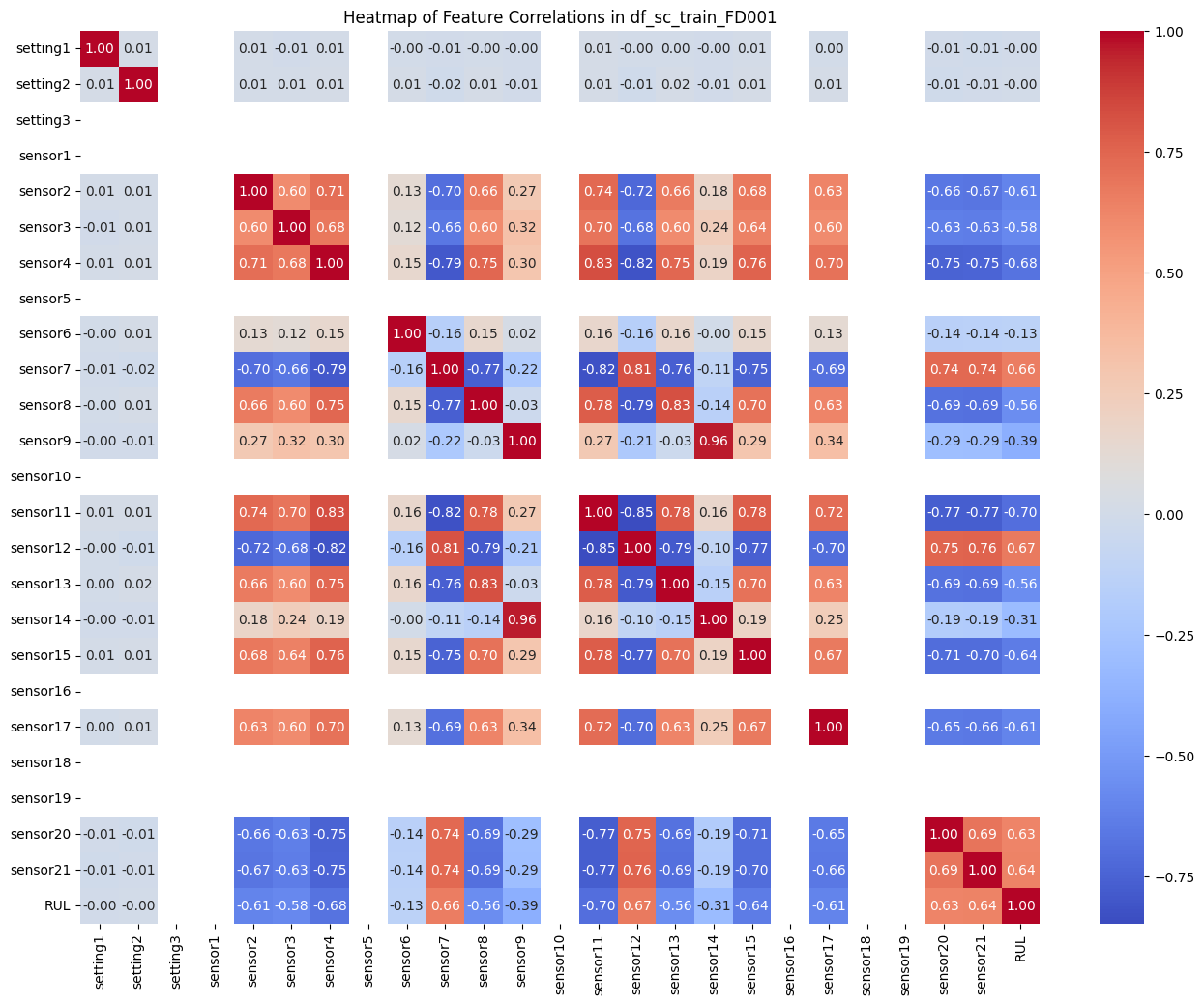
To extract useful features from the data, we explored heatmaps and conducted correlation analysis. We specifically investigated correlations within two ranges: above 0.4 or below -0.4, and above 0.6 or below -0.6. The results showed better metrics in correlations above 0.6 or below -0.6, indicating stronger relationships among the variables.
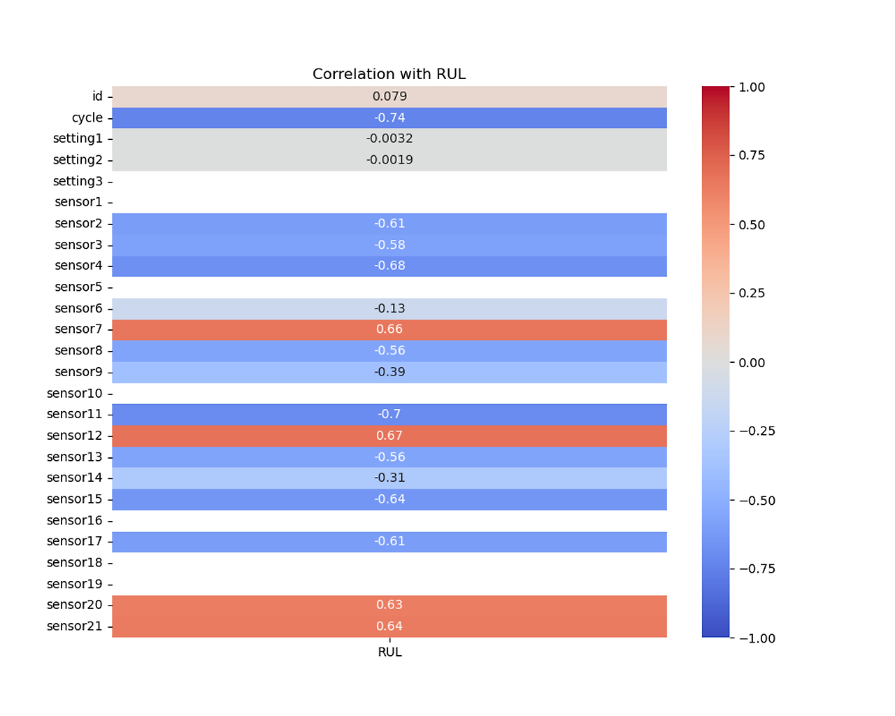
RUL stands for Remaining Useful Life, calculated as max cycle - cycle. I added a RUL column and proceeded with machine learning based on this. I compared the MSE and R2 score among the two groups and finally decided to select the columns 'sensor2', 'sensor4', 'sensor7', 'sensor11', 'sensor12', 'sensor15', 'sensor17', 'sensor20', and 'sensor21', which have correlations above 0.6 or below -0.6.
-
# Define RUL calculation function
def calculate_rul(data):
    # Calculate max(cycle) for each id
    max_cycles = data.groupby('id')['cycle'].max().reset_index()
    max_cycles.columns = ['id', 'max_cycle']
    # Merge max(cycle) back to the original data
    merged_data = data.merge(max_cycles, on='id')
    # Calculate RUL
    merged_data['RUL'] = merged_data['max_cycle'] - merged_data['cycle']
    return merged_data

# Calculate RUL for FD001 training dataset
df_train_FD001 = calculate_rul(df_train_FD001)

# Merge actual RUL for FD001 test dataset
df_rul_FD001.columns = ['RUL']
df_test_FD001 = df_test_FD001.groupby('id').last().reset_index()
df_test_FD001['RUL'] = df_rul_FD001['RUL']

# Select desired columns
selected_columns = ['sensor2', 'sensor4', 'sensor7', 'sensor11', 'sensor12', 'sensor15', 'sensor17', 'sensor20', 'sensor21']
X_train = df_train_FD001[selected_columns]
y_train = df_train_FD001['RUL']
X_test = df_test_FD001[selected_columns]
y_test = df_test_FD001['RUL']
-
# Train Linear Regression model
model = LinearRegression()
model.fit(X_train, y_train)

# Predict
y_pred_train = model.predict(X_train)
y_pred_test = model.predict(X_test)

# Evaluate model performance
train_mse = mean_squared_error(y_train, y_pred_train)
test_mse = mean_squared_error(y_test, y_pred_test)
train_r2 = r2_score(y_train, y_pred_train)
test_r2 = r2_score(y_test, y_pred_test)

print(f'Train MSE: {train_mse}, Train R^2: {train_r2}')
print(f'Test MSE: {test_mse}, Test R^2: {test_r2}')

#result
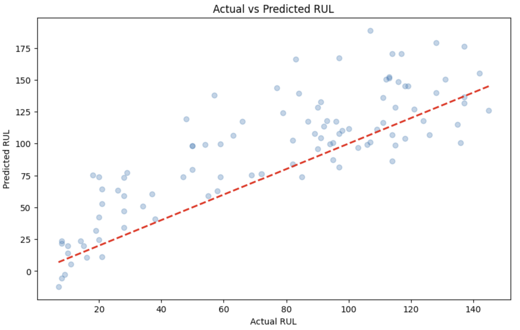
Train MSE: 2133.5726349674173, Train R^2: 0.5502928482652942
Test MSE: 1039.1683432855525, Test R^2: 0.39823577687304657
-
# Graph
plt.figure(figsize=(10, 6))
plt.scatter(y_test, y_pred_test, alpha=0.3)
plt.plot([y_test.min(), y_test.max()], [y_test.min(), y_test.max()], 'r--', lw=2)
plt.xlabel('Actual RUL')
plt.ylabel('Predicted RUL')
plt.title('Actual vs Predicted RUL')
plt.show()
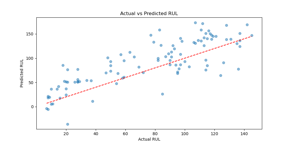
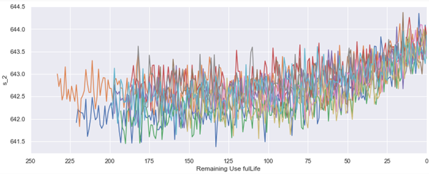
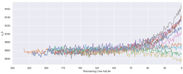
Based on this data, we examined the numerical values for each sensor and discovered that fluctuations in the values start occurring after 125. Using this observation, we decided to employ clipping to limit the variability from 125 to 0, making it suitable for machine learning and deep learning applications.


Model Evaluation and Performance Improvement
PCA and Correlation 0.6: Train MSE, Test MSE, Train R², Test R², Train Error, Test Error
| Linear Regerssion | 437.002 | 511.763 | 0.748 | 0.681 | 0.44 | 0.48 |
| SVM Regression | 341.681 | 516.239 | 0.803 | 0.679 | 0.15 | 0.23 |
| Ridge Regerssion | 437.002 | 511.762 | 0.748 | 0.681 | 0.44 | 0.48 |
| Lasso Regerssion | 439.628 | 505.660 | 0.747 | 0.685 | 0.43 | 0.47 |
| Elasticnet | 445.190 | 502.390 | 0.744 | 0.687 | 0.43 | 0.489 |
| Random Forest Regerssion | 331.300 | 363.131 | 0.810 | 0.773 | 0.43 | 0.37 |
| XGboost | 196.838 | 443.188 | 0.887 | 0.724 | 0.21 | 0.30 |
Without PCA and Correlation 0.6: Train MSE, Test MSE, Train R², Test R², Train Error, Test Error
| Linear Regerssion | 436.105 | 506.359 | 0.749 | 0.685 | 0.43 | 0.48 |
| SVM Regression | 324.508 | 422.475 | 0.813 | 0.737 | 0.14 | 0.20 |
| Ridge Regerssion | 436.105 | 506.359 | 0.745 | 0.685 | 0.43 | 0.48 |
| Lasso Regerssion | 436.105 | 506.357 | 0.749 | 0.685 | 0.43 | 0.48 |
| Elasticnet | 442.013 | 500.383 | 0.745 | 0.688 | 0.43 | 0.48 |
| Random Forest Regerssion | 306.692 | 365.040 | 0.823 | 0.772 | 0.30 | 0.32 |
| XGboost | 242.051 | 402.707 | 0.861 | 0.749 | 0.22 | 0.29 |
With PCA and Correlation 0.4: Train MSE, Test MSE, Train R², Test R², Train Error, Test Error
| Linear Regerssion | 430.091 | 504.721 | 0.752 | 0.686 | 0.43 | 0.47 |
| SVM Regression | 324.034 | 398.009 | 0.813 | 0.752 | 0.14 | 0.20 |
| Ridge Regerssion | 430.091 | 504.720 | 0.752 | 0.686 | 0.43 | 0.47 |
| Lasso Regerssion | 435.657 | 491.160 | 0.750 | 0.694 | 0.42 | 0.46 |
| Elasticnet | 441.968 | 487.210 | 0.746 | 0.697 | 0.42 | 0.47 |
| Random Forest Regerssion | 337.283 | 385.198 | 0.806 | 0.760 | 0.41 | 0.35 |
| XGboost | 302.013 | 401.557 | 0.83 | 0.75 | 0.27 | 0.30 |
Without PCA and Correlation 0.4: Train MSE, Test MSE, Train R², Test R², Train Error, Test Error
| Linear Regerssion | 427.402 | 498.591 | 0.754 | 0.690 | 0.43 | 0.46 |
| SVM Regression | 281.710 | 330.550 | 0.838 | 0.794 | 0.13 | 0.17 |
| Ridge Regerssion | 427.402 | 498.590 | 0.754 | 0.690 | 0.43 | 0.46 |
| Lasso Regerssion | 427.439 | 498.543 | 0.754 | 0.690 | 0.43 | 0.46 |
| Elasticnet | 437.469 | 489.685 | 0.748 | 0.695 | 0.13 | 0.48 |
| Random Forest Regerssion | 292.807 | 356.009 | 0.831 | 0.778 | 0.28 | 0.30 |
| XGboost | 269.764 | 342.671 | 0.845 | 0.787 | 0.24 | 0.26 |
Base Train MSE, Test MSE, Train R², Test R², Train Error, Test Error
| Linear Regerssion | 398.697 | 458.826 | 0.770 | 0.714 | 0.48 | 0.45 |
| SVM Regression | 324.508 | 422.470 | 0.813 | 0.737 | 0.14 | 0.20 |
| Ridge Regerssion | 339.222 | 458.798 | 0.770 | 0.714 | 0.48 | 0.46 |
| Lasso Regerssion | 398.714 | 458.645 | 0.770 | 0.714 | 0.48 | 0.45 |
| Elasticnet | 400.269 | 456.870 | 0.770 | 0.715 | 0.48 | 0.45 |
| Random Forest Regerssion | 213.268 | 265.786 | 0.877 | 0.834 | 0.22 | 0.25 |
| XGboost | 238.424 | 260.508 | 0.863 | 0.838 | 0.22 | 0.23 |
With PCA and Correlation 0.4 and Smoothing: Train MSE, Test MSE, Train R², Test R², Train Error, Test Error
| Linear Regerssion | 488.881 | 1316.663 | 0.718 | 0.180 | 0.47 | 1.14 |
| SVM Regression | 378.290 | 1315.630 | 0.782 | 0.181 | 0.15 | 0.41(?) |
| Ridge Regerssion | 488.881 | 1316.663 | 0.718 | 0.180 | 0.47 | 1.14 |
| Lasso Regerssion | 488.881 | 1316.663 | 0.718 | 0.180 | 0.47 | 1.14 |
| Elasticnet | 488.881 | 1316.665 | 0.718 | 0.180 | 0.47 | 1.14 |
| Random Forest Regerssion | 343.747 | 1284.097 | 0.802 | 0.200 | 0.40 | 1.05 |
| XGboost | 126.178 | 1385.408 | 0.927 | 0.137 | 0.18 | 1.07 |
With PCA and Correlation 0.6 and Smoothing: Train MSE, Test MSE, Train R², Test R², Train Error, Test Error
| Linear Regerssion | 507.990 | 1335.150 | 0.707 | 0.168 | 0.48 | 1.13 |
| SVM Regression | 407.633 | 1369.051 | 0.765 | 0.147 | 0.16 | 0.42 |
| Ridge Regerssion | 507.990 | 1335.151 | 0.707 | 0.168 | 0.48 | 1.13 |
| Lasso Regerssion | 507.990 | 1335.155 | 0.707 | 0.168 | 0.48 | 1.13 |
| Elasticnet | 507.990 | 1335.160 | 0.707 | 0.168 | 0.48 | 1.13 |
| Random Forest Regerssion | 359.106 | 1310.714 | 0.793 | 0.183 | 0.42 | 1.01 |
| XGboost | 111.032 | 1265.155 | 0.936 | 0.212 | 0.17 | 0.96 |
Without PCA and Correlation 0.4 and Smoothing: Train MSE, Test MSE, Train R², Test R², Train Error, Test Error
| Linear Regerssion | 486.630 | 1341.011 | 0.719 | 0.164 | 0.47 | 1.15 |
| SVM Regression | 378.290 | 1315.630 | 0.782 | 0.180 | 0.15 | 0.41 |
| Ridge Regerssion | 486.630 | 1341.009 | 0.719 | 0.164 | 0.47 | 1.15 |
| Lasso Regerssion | 495.970 | 1327.997 | 0.714 | 0.173 | 0.48 | 1.14 |
| Elasticnet | 495.368 | 1332.623 | 0.714 | 0.170 | 0.48 | 1.14 |
| Random Forest Regerssion | 215.676 | 1332.409 | 0.875 | 0.170 | 0.21 | 1.07 |
| XGboost | 90.069 | 1392.484 | 0.948 | 0.132 | 0.14 | 1.07 |
Without PCA and Correlation 0.6 and Smoothing: Train MSE, Test MSE, Train R², Test R², Train Error, Test Error
| Linear Regerssion | 505.066 | 1340.537 | 0.709 | 0.165 | 0.48 | 1.14 |
| SVM Regression | 378.290 | 1315.629 | 0.782 | 0.181 | 0.15 | 0.41 |
| Ridge Regerssion | 505.066 | 1340.537 | 0.709 | 0.165 | 0.48 | 1.14 |
| Lasso Regerssion | 506.124 | 1339.176 | 0.708 | 0.166 | 0.48 | 1.13 |
| Elasticnet | 506.432 | 1338.855 | 0.708 | 0.166 | 0.48 | 1.14 |
| Random Forest Regerssion | 282.846 | 1374.486 | 0.837 | 0.144 | 0.25 | 1.02 |
| XGboost | 58.721 | 1491.978 | 0.966 | 0.070 | 0.11 | 1.03 |
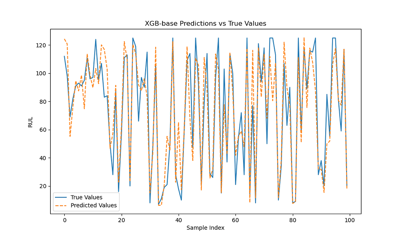
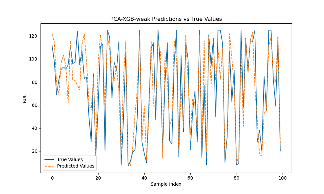
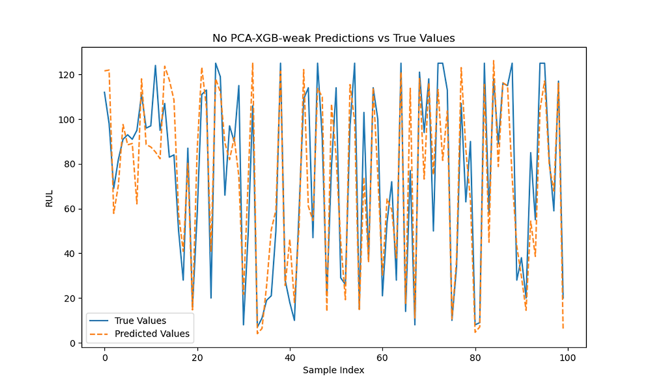
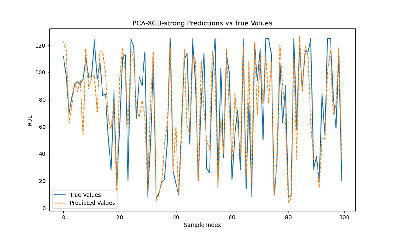
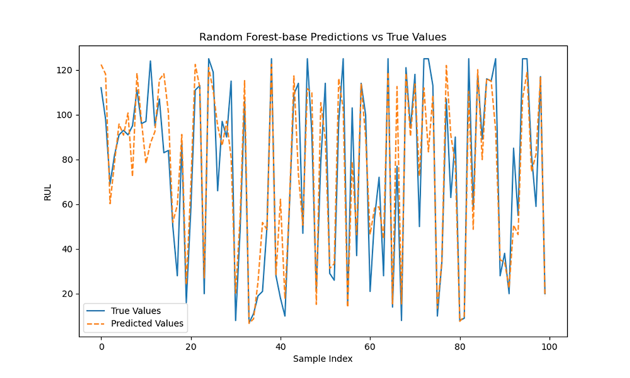
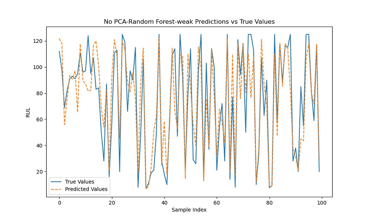
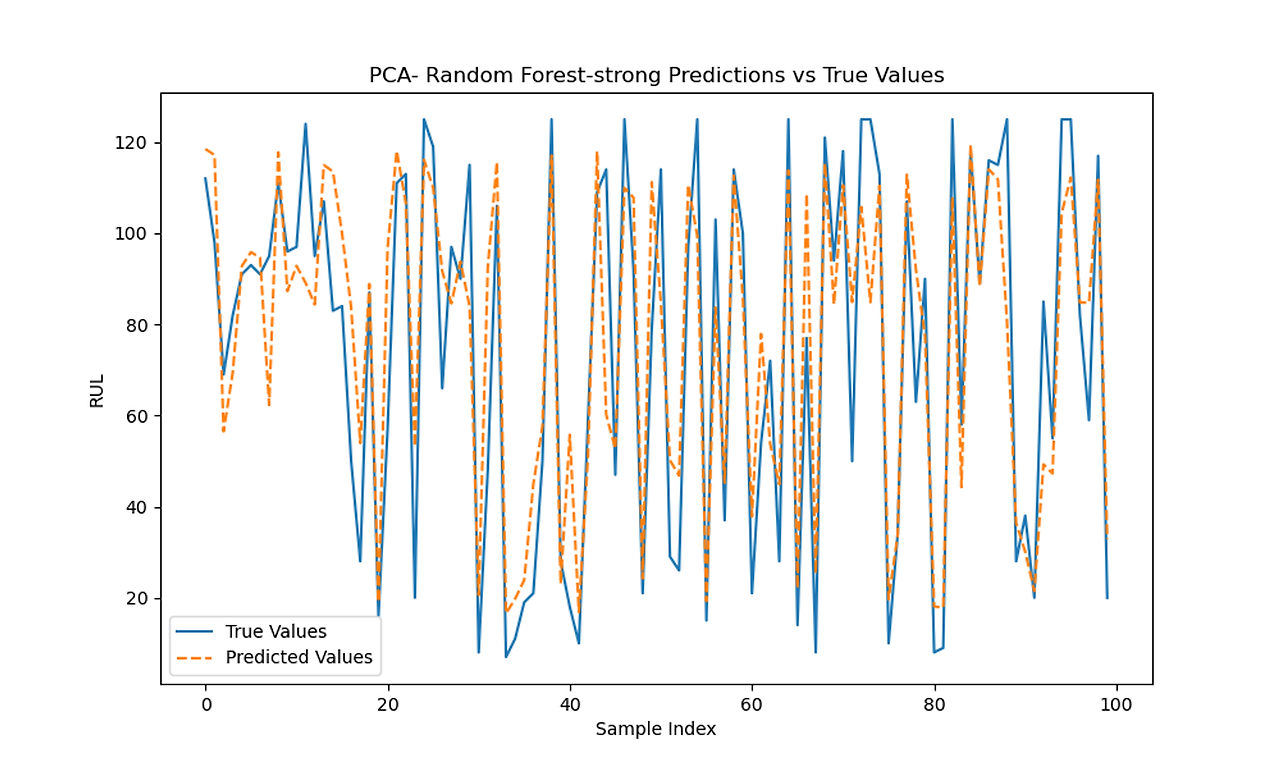
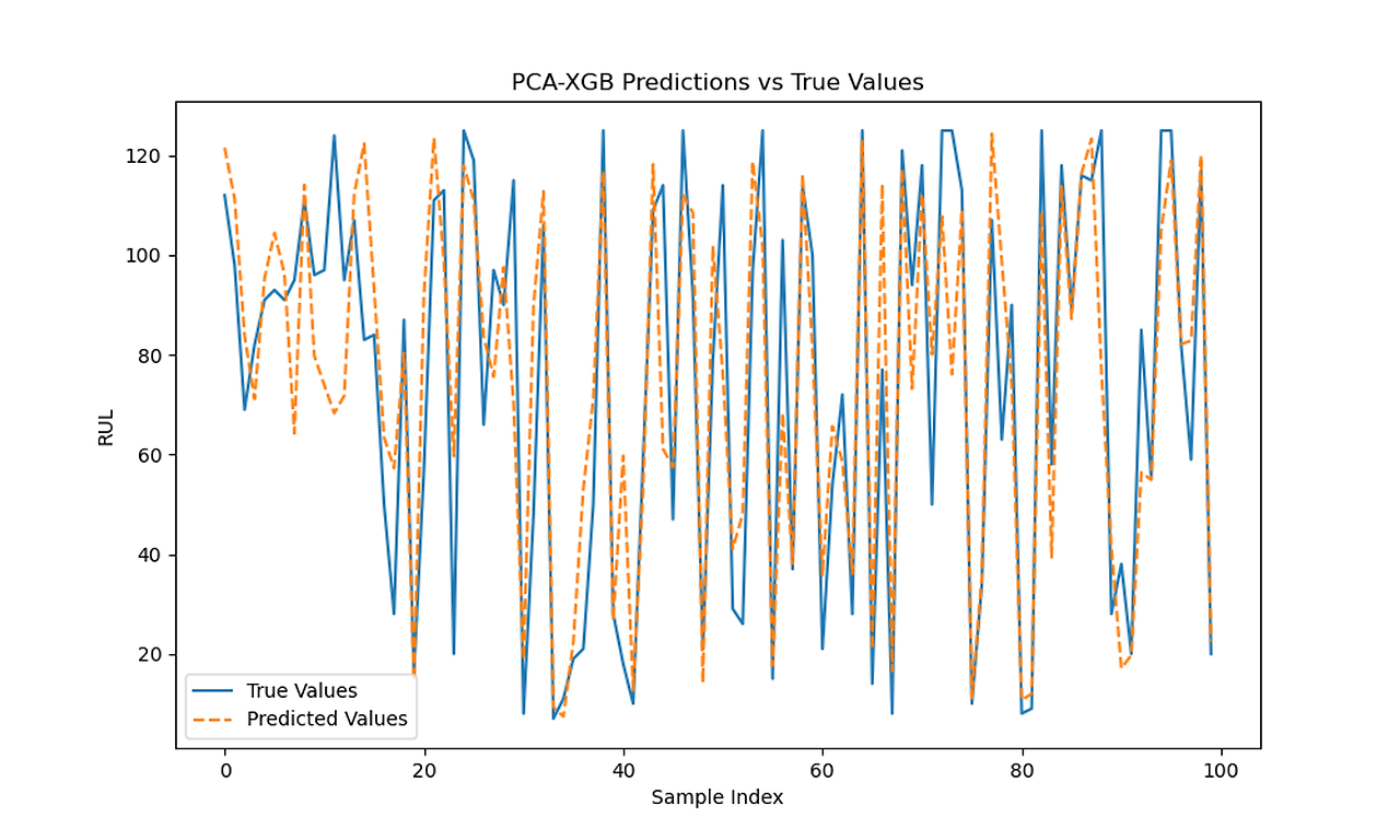
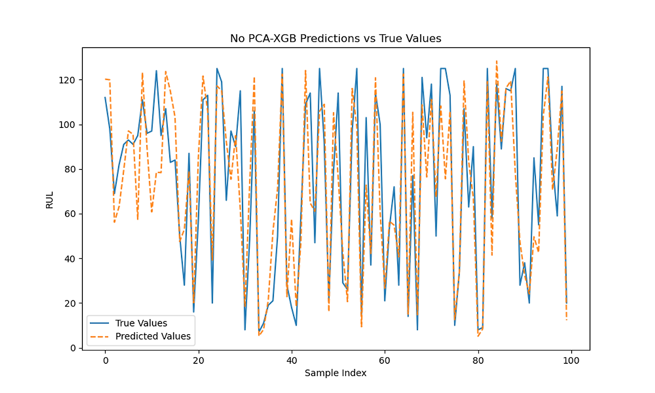
XGB 0.4 Predictions vs Actual with and without PCA

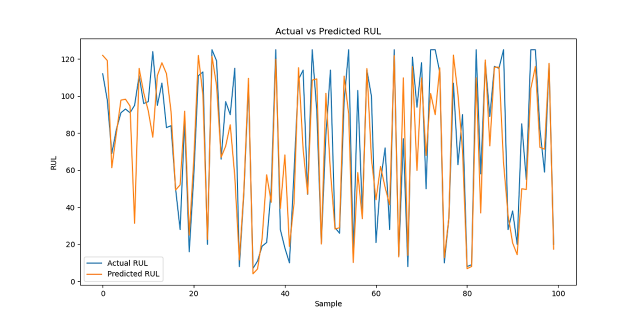
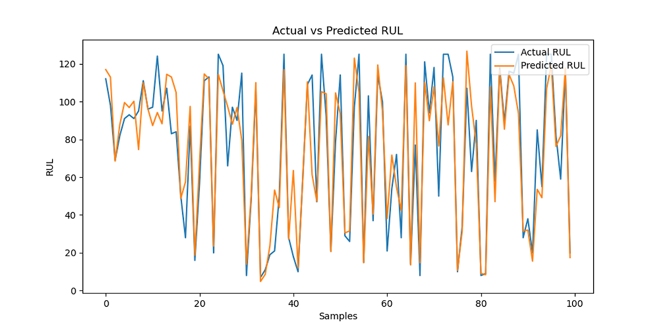
LSTM RUL Predictions vs Actual RUL
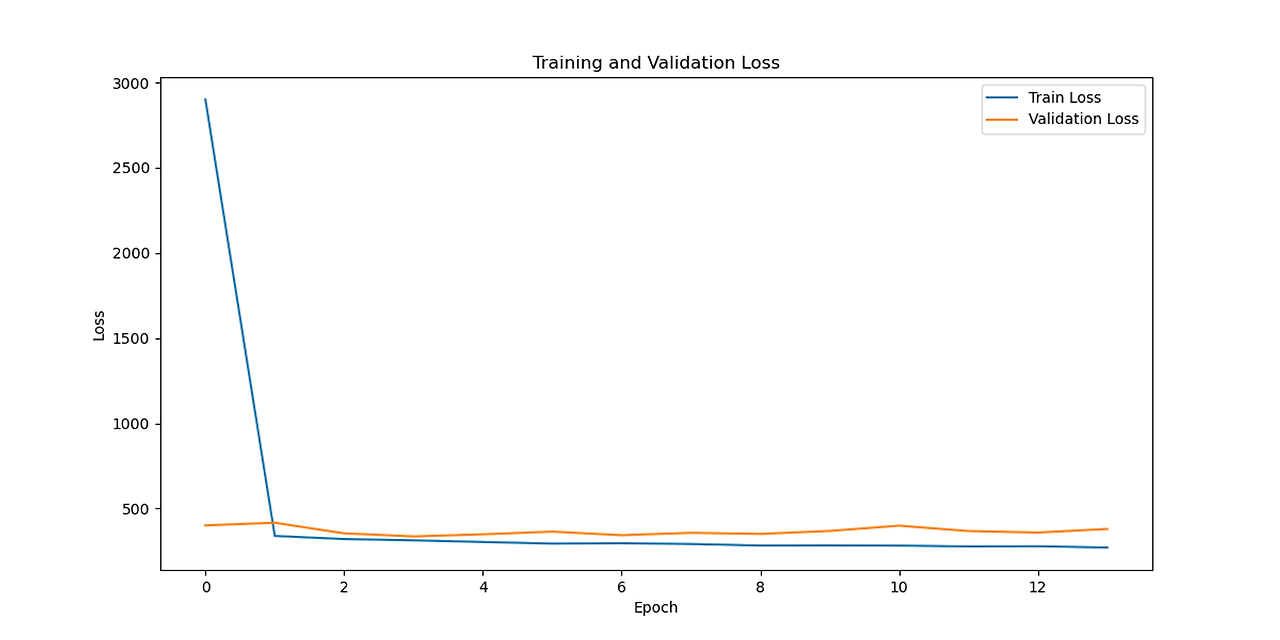
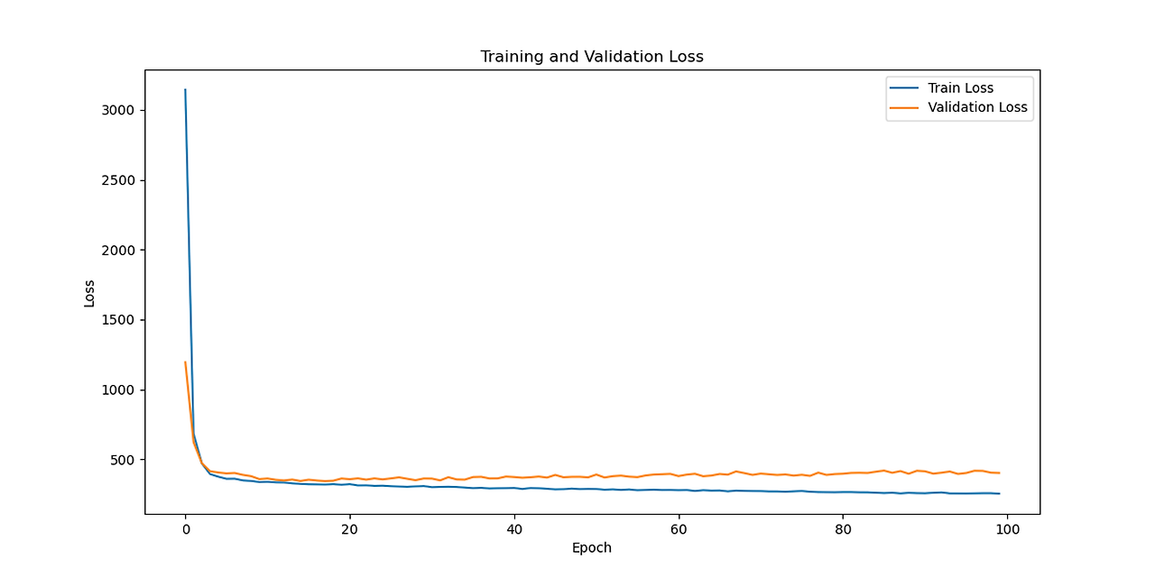
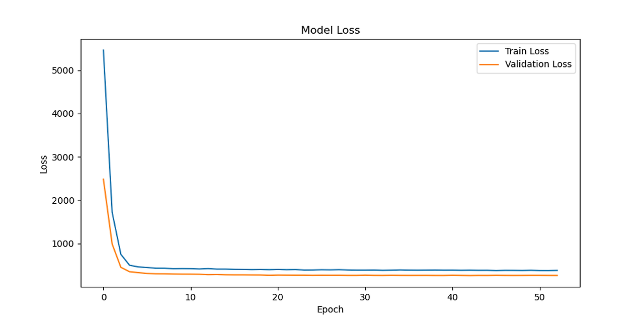
LSTM model loss
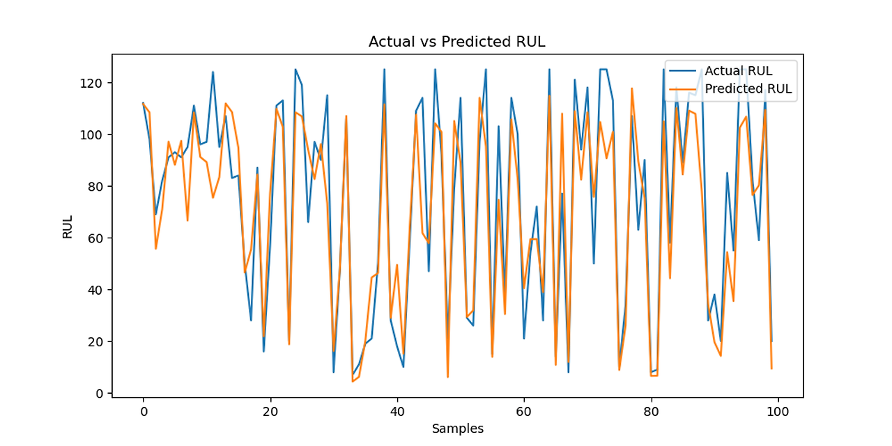
CNN-LSTM Predictions vs Actual RUL
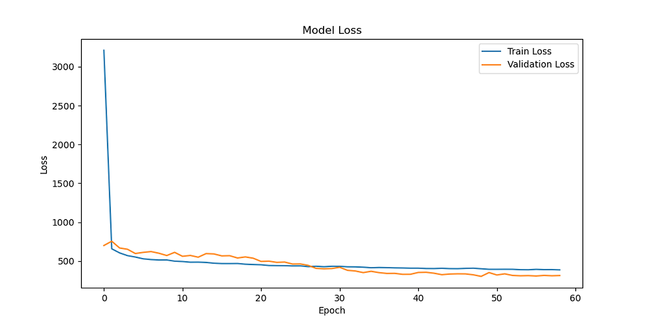
CNN-LSTM loss
Transformer-LSTM Predictions vs Actual

Transformer-LSTM loss
